Phasors

Phasors

Rotating vectors, known as a phasors, can be used to analyse diffraction patterns

Ron Holt

 

The wave nature of light and how it diffracts through a single slit and interferes through multislits can be explained using a special type of vector called a phasor.

Consider the case of adding two sine waves together, which have identical frequencies (f) and amplitudes (A) but differ only in phase, φ. If the phase difference is zero then the two waves add together to give a resultant wave that has the same frequency but now double the amplitude (this is called constructive interference). If the phase difference is 180° (π radians) then the two waves cancel each other out and there is no resultant wave (this is called destructive interference).

In between these extremes there is a continuous range of intermediate amplitudes and hence intensities, where the intensity is proportional to the square of the resultant amplitude.

However, calculating the resultant wave amplitude at these intermediate values becomes a rather tedious process, and adding together three or more sine waves soon becomes impracticable.

Phasors

An alternative and more efficient method is to replace each of the sine waves by an anticlockwise rotating arrow, called a phasor, that completes one cycle within the same time period as the wave. At any stage in a cycle the amplitude of the wave is defined by the projection of the arrow onto the y-axis. The phasor has both magnitude and direction and, just like a vector, allows any number of waves to be added together by vector addition.

A sinusoidal wave (sine wave) with an amplitude A, frequency f and zero initial phase can be represented by a displacement y, at time t:

y = A sin (2πft)

= A sin (ωt) (1)

Often ω is referred to as the angular frequency.

Alternatively the displacement can be shown as a rotating arrow of length A undergoing uniform circular motion with angular frequency ω in an anticlockwise direction (Figure 1).

 

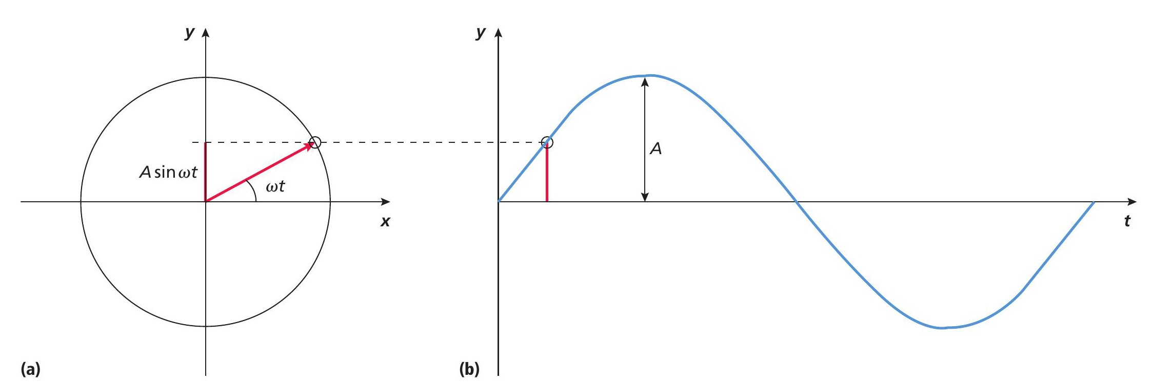
The zero initial phase shows an arrow that is horizontal and pointing in the positive direction. The rotating arrow keeps track of where a wave is in its cycle so that the direction of the arrow gives the phase, whilst its displacement A sin (ωt) gives the amplitude. This rotating arrow is what we call a phasor.

Superposition of three phasors

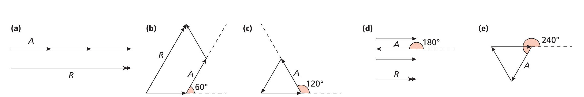
Take the superposition of three identical sine waves (all with frequency f and amplitude A), using phasor addition, where the phase difference between one phasor and the next is φ.

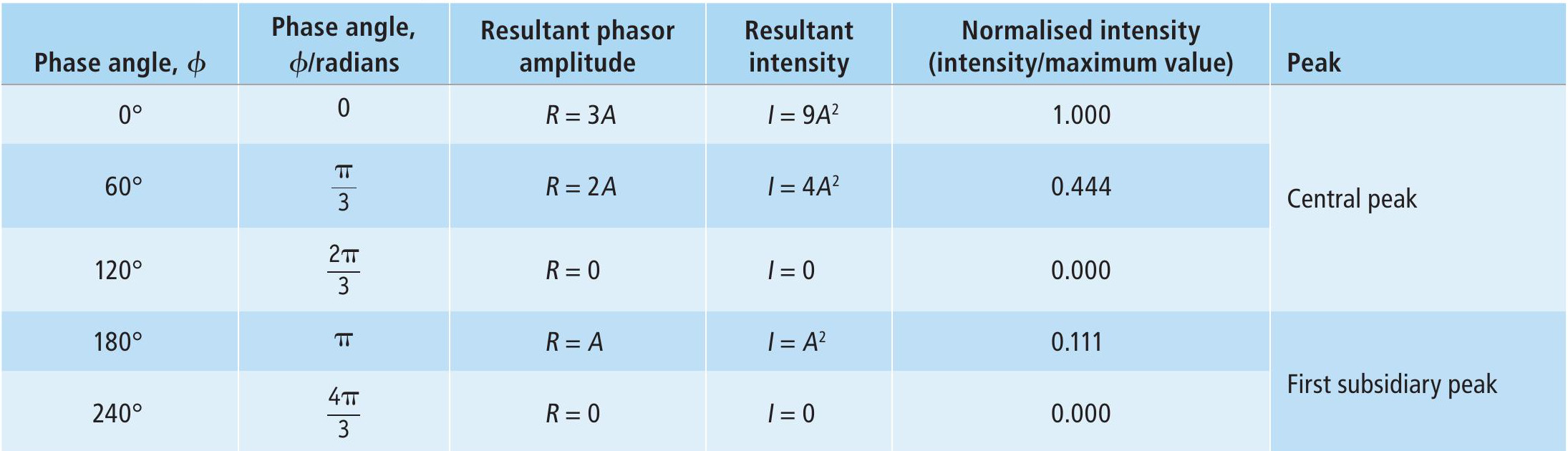
When φ = 0° constructive interference gives a resultant amplitude R and intensity I:

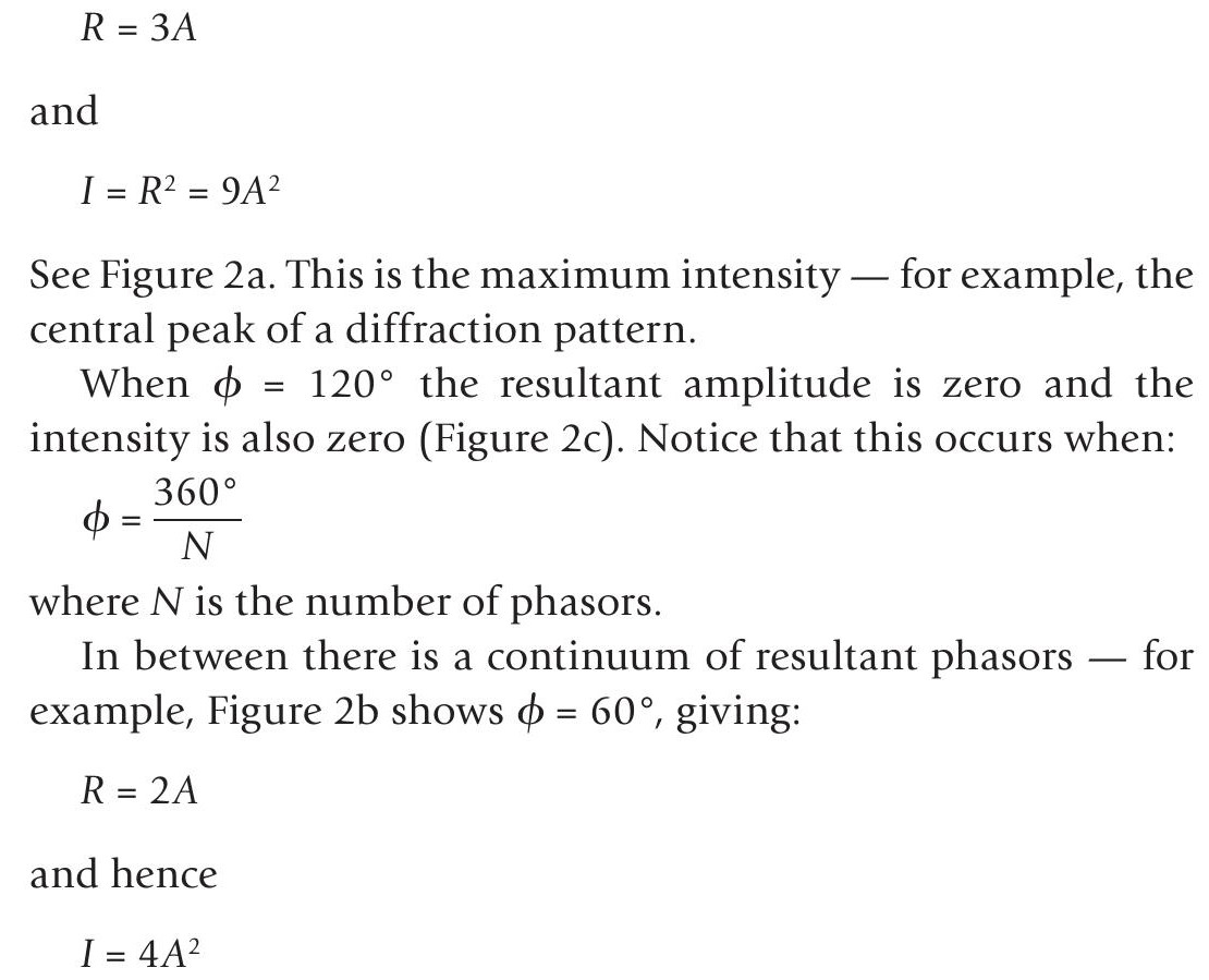
When the overall phase angle between the first and last phasors goes beyond 360° there is a subsidiary maximum. In our example with three phasors, this is when φ is over 120°: there is a maximum intensity of I = A2at φ = 180° (Figure 2d) and the amplitude falls to zero again when when φ = 240° (Figure 2e).

Table 1 summarises these results.

Generalisation of the phasor model

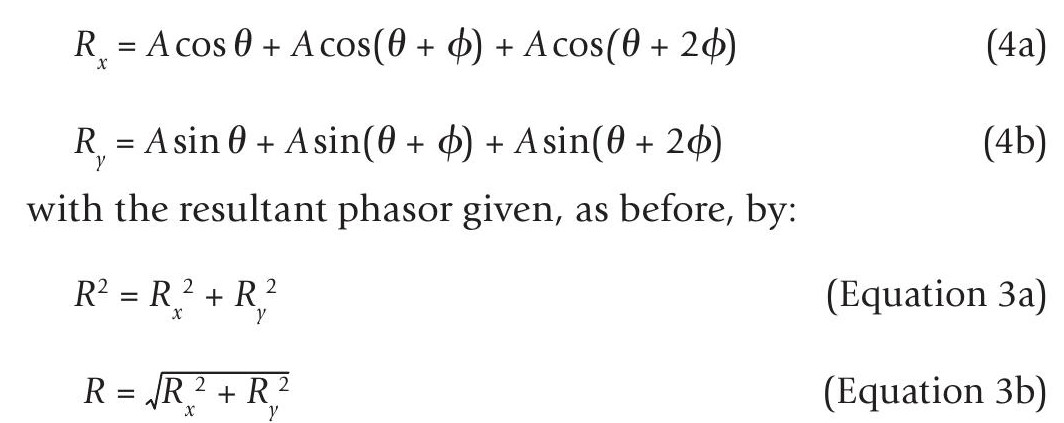
In order to generalise the model for a complete range of phase angles we express the phasor in terms of its x and y components (PHYSICS REVIEW Vol. 31, No. 4, pp. 12–15) and use the rules of standard trigonometry.

For the three-wave phasor model in Figure 3:

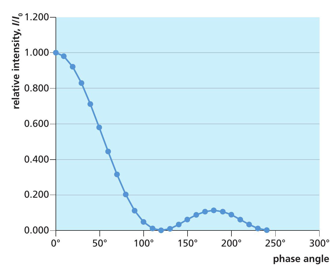
Figure 4 shows the resultant intensity, I, for the three-wave phasor model based on the above expressions, given as a fraction of the maximum intensity I0 (the intensity of the central peak). Since only three wave superpositions are involved, only the first subsidiary peak is observed. Higher-order peaks are obtained when the phasor model goes beyond seven or more superpositions.

Application to single-slit diffraction

The phasor model is ideally suited to describe the effects of single-slit diffraction and multislit interference.

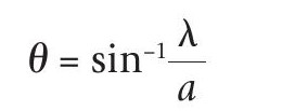
Think about diffraction by a single slit. Coherent light, of wavelength λ, passing through a single slit, width a, is diffracted in all directions. This light interferes both constructively (to form bright bands) and destructively (to form dark bands) on a screen a distance D from the slit. The resultant difference in path length from light emitted from either side of the slit is a function of a sin θ, where θ is the angle from the straight-through direction, as shown in Figure 5. This results in a broad maximum bright band at θ = 0° followed by a narrow dark band at:

Diffraction experiments are usually performed using red laser light with wavelength 635 nm, while a typical slit width is 1.59 µm, equivalent to 2.5 λ. This gives θ = 11.5° for the first zero. A second but less intense bright band appears at θ = 17.4°, while a second narrow, dark band appears when θ = 24.6°.

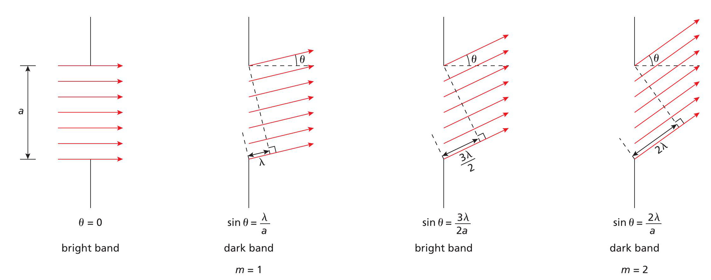
Figure 6a shows a single-slit diffraction pattern produced with a red laser, and Figure 6b shows the diffraction pattern generated using a three-wave phasor model (i.e. N = 3), combining waves from the centre and both edges of the slit. The calculations were performed using a spreadsheet.

For each diffraction angle, θ, the corresponding path difference (and hence phase difference, φ) was determined using a modified version of Equation 2:

The calculated diffraction pattern shows diffraction minima at 12° and 24°. The central maximum is twice the width of the subsidiary peaks, and the narrow, dark bands are accurately located.

If a more accurate simulation of a single-slit diffraction pattern is to emerge then more waves in the phasor model are needed — in reality, the number of waves that interfere is infinite. As shown in Box 1, we can generalise Equations 4a and 4b to include any number of waves, N. Figures 7b and 7c show the results for a 13-wave phasor model (13 terms in each component). For comparison, Figure 7a shows the single-slit diffraction pattern extended to show three subsidiary bright bands. Note that the widths of the diffraction peaks are all half the width of the central peak, which has a width 2 λ D/a.

Peak intensities

In practice it is often difficult to discern the third or even the second bright band beyond the central band, as depicted in Figure 7. Suppose the central bright band has an amplitude A0 and intensity I0= A02. Then the first subsidiary bright peak amplitude is:

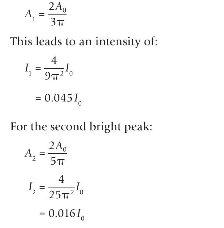
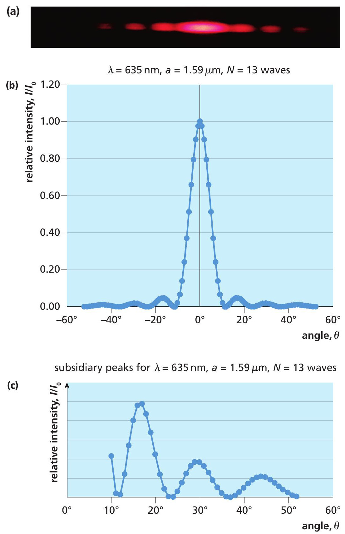
The precise positions of these bands and the intensity levels of the bright bands can be determined by looking in more detail at the low-intensity end of the pattern, as shown in Figure 7c.

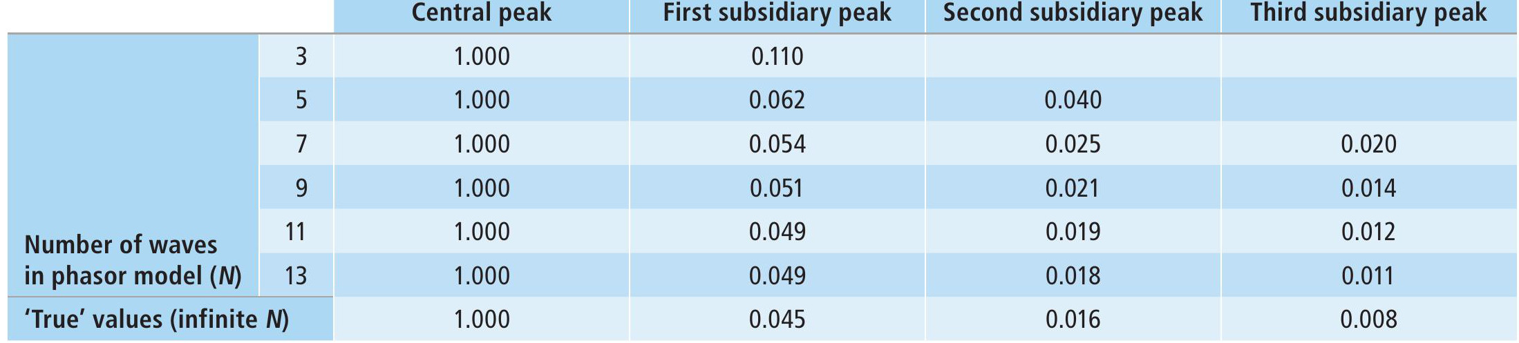
Table 2 shows the calculated peak intensities up to the third subsidiary peak under the conditions set above, along with the ‘true’ peak intensities calculated using an infinite number of interfering waves. As more waves are included in the model then the closer the model is to reality. The phasor model as expressed by the spreadsheet can be readily adapted to vary both wavelength and slit width, as well as to simulate both double-slit and diffraction grating phenomena.

Conclusion

While this article might have taken you beyond the requirements of your A-level (or equivalent) course, I hope it has helped you to visualise the physics underlying single-slit diffraction patterns, and to appreciate some neat mathematical analysis that you might explore further if you pursue your studies of physics to a higher level.

Ron Holt is a physicist, author and teacher.