Measuring the speed of sound

SKILLSET

Measuring the speed of sound

Ian Lovat discusses how to measure the speed of sound in air using a double-beam oscilloscope

 

The exam boards for A-level physics require or suggest a number of practical activities that will allow you to satisfy the Common Practical Assessment Criteria (CPACs). Among other requirements, you are expected to be able to make accurate observations relevant to the experiment, to obtain accurate, precise and sufficient data, and record these methodically using correct units and conventions, and to use ICT with appropriate software to process data.

The straightforward experiment discussed in this Skillset uses an oscilloscope (in this case a PC-based one) and a signal generator (also PC-based) to measure the speed of sound by measuring the wavelengths of different frequencies of sound in air.

A different method of measuring the speed of sound — by finding the wavelength of stationary waves in a resonance tube — was covered in Physics Review Vol. 32, No. 2, Exam talkback .

Background

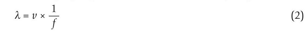
The frequency, f, and wavelength, λ, of any wave are linked by the wave equation:

where v is the speed of the wave through the medium. Rearranging Equation 1 to make λ the subject gives:

Comparing Equation 2 with the equation for a straight line

y = mx + c

it can be seen that by measuring the wavelengths for different frequencies of sound and plotting a graph of λ against 1/f, the gradient, m, is equal to the speed of the wave, v:

Experimental arrangement

The experimental arrangement is shown in Figure 1, and the Resources box gives details of videos showing the experiment being carried out.

 

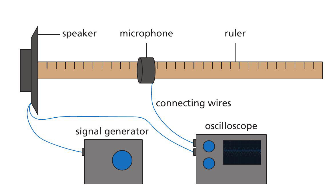
A signal generator is connected to a small loudspeaker, which is mounted vertically. The signal that goes to the speaker is also connected to one input of a double-beam oscilloscope. The second beam of the oscilloscope is connected to a microphone, which can be moved along a ruler.

There are various pieces of equipment that can be used for the oscilloscope and signal generator, including a standard analogue signal generator and dual-beam oscilloscope, but for this particular experimental arrangement the signal generator was a digital signal generator on a PC using a free program called Audacity (see Resources box). Other programs able to generate a fixed tone are available.

The double-beam oscilloscope was a USB-connected PC-based oscilloscope. Both the signal generator and oscilloscope were running on the same PC.

If a standard laboratory analogue signal generator is used, the frequencies will need to be measured each time, either using the timebase of the oscilloscope or a digital frequency meter.

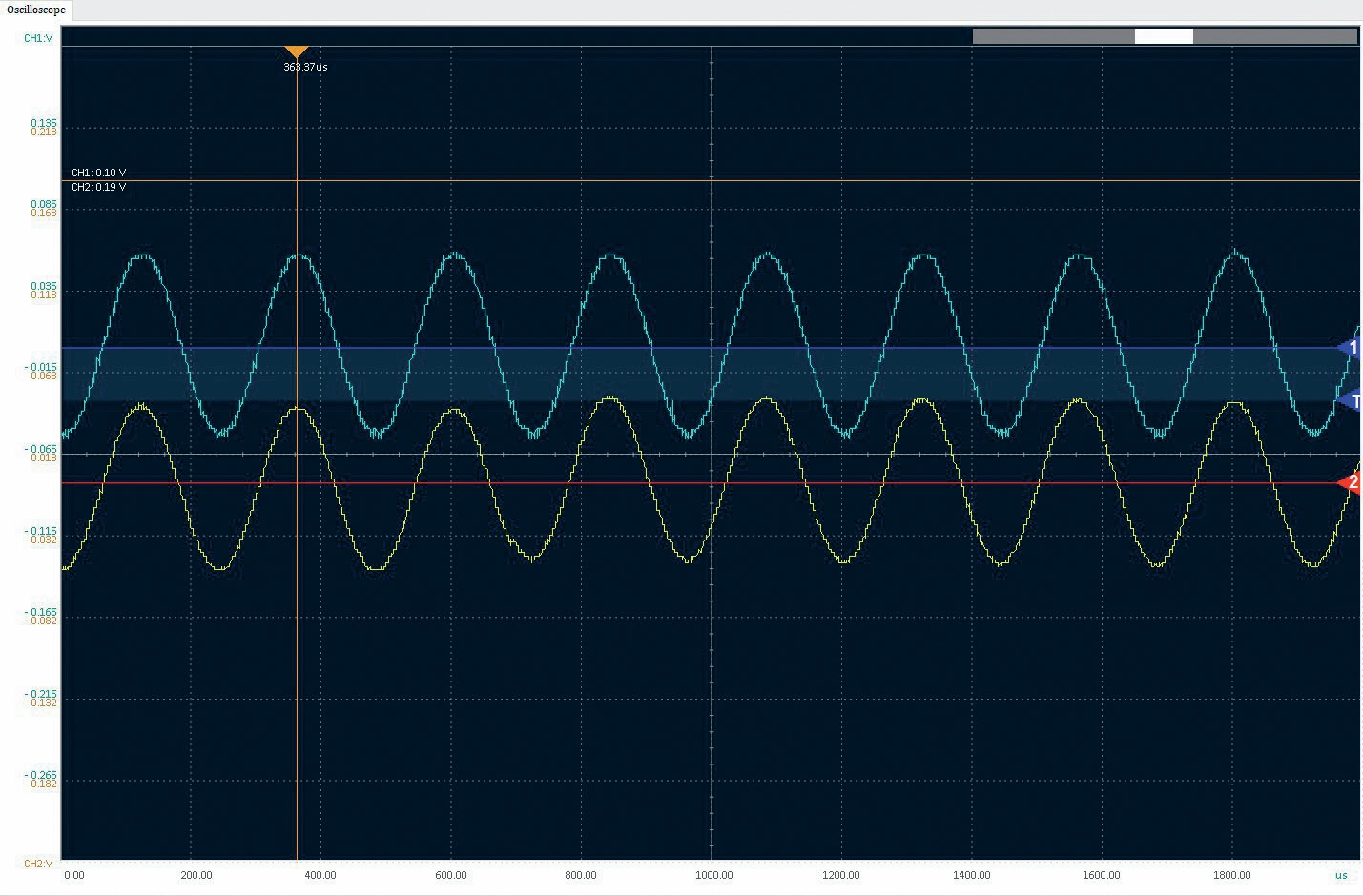
The loudspeaker is connected to the signal generator and to one beam of the oscilloscope. The oscilloscope is adjusted to give a clear waveform on screen with the triggering set to the channel connected to the speaker (Figure 2).

The microphone is connected to the second channel and placed in front of the speaker. It is then moved backwards or forwards until the waveforms on the screen align exactly. On the PC-based oscilloscope this is made easier with the use of the cursor. At this point, there is a whole number of waves between the speaker and the microphone. The position of the microphone on the ruler is noted.

The microphone is then moved away from the speaker while noting that, as the microphone is moved, the microphone waveform moves to the right on the oscilloscope screen. It is moved until a subsequent wave exactly aligns again. For each adjacent wave that aligns, the microphone has been moved by one wavelength. In this experiment, it was possible to move the microphone two complete waves while still having a measurable and reliable trace on the oscilloscope screen. However, depending on the amplitude of the signal from the speaker and the sensitivity of the microphone, it may be possible to move the microphone more than two complete waves.

The frequency of the signal to the loudspeaker is changed and the procedure repeated until five or six measurements have been taken. The range of frequencies used in this case was between 2.5 kHz and 5.0 kHz. These frequencies give wavelengths that are easily measurable on a metre ruler.

Recording results

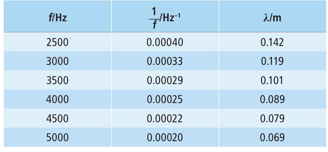
A typical set of results is shown in Table 1.

A graph is drawn of wavelength against 1/f, as shown in Figure 3. The gradient, m, of this graph is the speed of sound in air.

Uncertainty and conclusion

In this experiment the tone generated can be set exactly — measurements with a frequency meter show it to be accurate to within ± 1.0 Hz. A further check using the oscilloscope timebase also shows the frequency to be accurate to within ± 1.0 Hz. This gives a maximum percentage uncertainty for all measurements of:

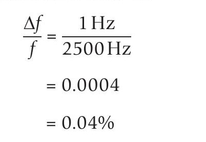
This is too small an uncertainty to show as error bars on the graph. However, when aligning the waveforms, the uncertainty in position for the microphone was found to be ± 2mm for each position or ± 4mm for the measurement of two wavelengths. This gives a maximum percentage uncertainty of 3% for the 5.0 kHz measurement, and therefore error bars corresponding to an uncertainty of ± 3% have been added to the graph for all points.

While it is possible to calculate the percentage uncertainty for each measurement, this is not necessary for A-level — only the maximum percentage uncertainty is needed.

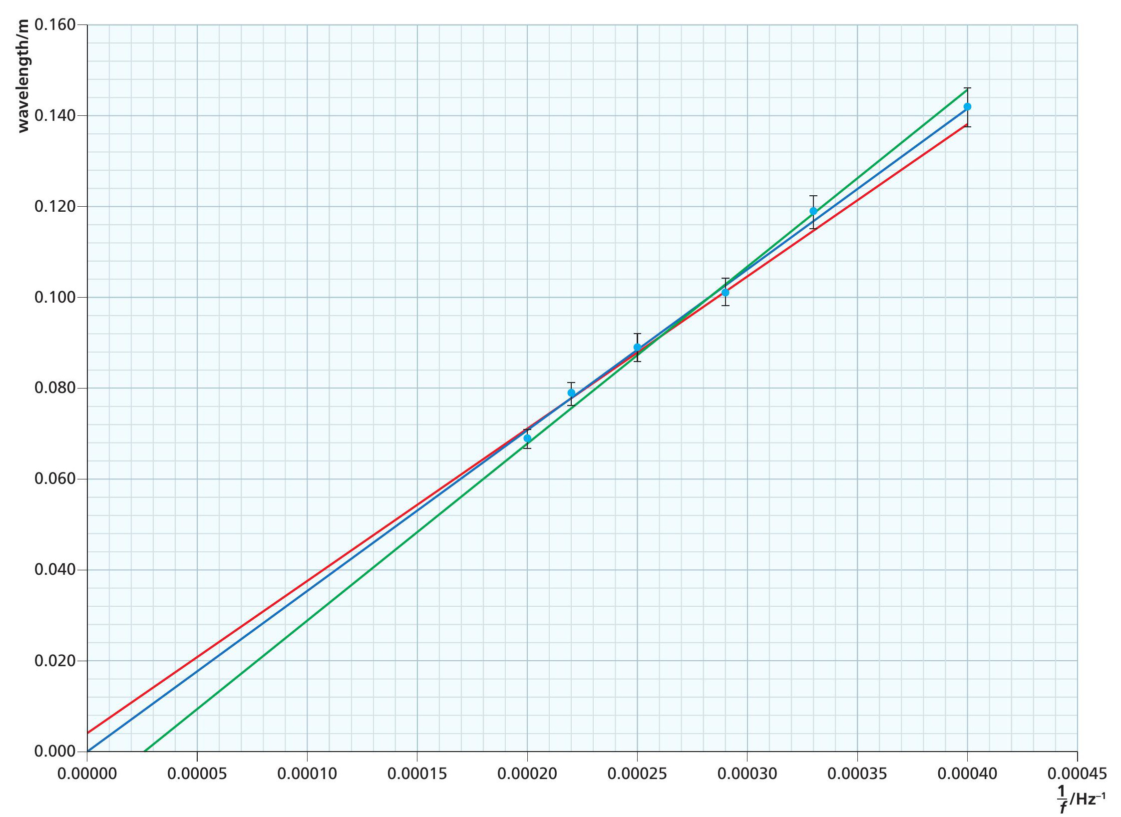
Standard graph-plotting software has been used to give the best-fit line (blue). The steepest (green) and shallowest (red) lines that also go through the error bars have been added (Figure 3).

The gradient of the best-fit line is:

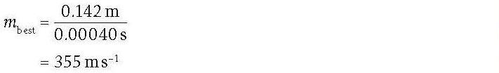
Therefore, from Equation 3:

vbest = 355 m s–1

The maximum gradient is:

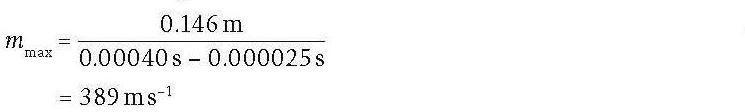
Therefore:

vmax = 389 m s–1

The minimum gradient is:

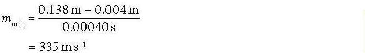
Therefore:

vmin = 335 m s–1

The range is:

vmax – vmin = 54 m s–1

Therefore the spread is 27ms–1.

The conclusion of this experiment is that the speed of sound is measured to be (355 ± 27)ms –1(± 8%)

Data tables give the speed of sound at sea level and 20°C as 343 m s–1, so the value obtained in this experiment includes the accepted value.

Ian Lovat is a former physics teacher and a member of the PHYSICS REVIEW editorial board.