SKILLSET
Calibrating a thermistor to measure temperature
Ian Lovat discusses how to calibrate a thermistor by measuring how the resistance changes with temperature
The exam boards for A-level physics require or suggest a number of practical activities that will allow you to satisfy the Common Practical Assessment Criteria (CPACs). Among other requirements, you are expected to be able to make accurate observations relevant to the experiment, to obtain accurate, precise and sufficient data, and record these methodically using correct units and conventions, and to use ICT with appropriate software to process data. Measuring the resistance of a thermistor at different temperatures gives practice in making careful measurements, while determining the relationship between resistance and temperature tests your ICT and analysis skills.
Background
A thermistor is an electronic component widely used wherever temperature sensing is required, for example digital thermometers, car sensors, sensors for medical use such as an incubator and for battery temperature sensing while charging and discharging. The resistance of the thermistor changes with temperature and in order to be useful we need to find a relationship between the resistance and temperature so that, for any given value of resistance, we can know the corresponding temperature. Described as calibrating the thermistor, this can be done either by finding a formula for the relationship or by reading values from a graph. For electronic equipment, finding a formula is the most useful as the formula can be programmed into the temperature recording or display circuit.
There are two main types of thermistor: an NTC (negative temperature coefficient) thermistor, in which the resistance falls as the temperature increases, and a PTC (positive temperature coefficient) thermistor, in which the resistance rises as the temperature increases.
Equations
The relationship between the resistance of a thermistor and temperature is non-linear. This is unlike the linear relationship between resistance RT at temperature T, which you may have encountered for a metallic conductor:
R = R0 (1 + αT)
where R0 is the resistance at 0°C and α is a constant.
Over a limited temperature range the resistance of a thermistor can be approximated to:
RT = R0 eαT (1)
where RT is the resistance at temperature T, R0 is the resistance at 0°C or 0K, depending on the unit used for the measurement of T, and α is a constant — called the temperature coefficient of resistance — specific to the thermistor used. It is negative for an NTC thermistor and positive for a PTC thermistor.
In order to be able to plot a straight-line graph of resistance against temperature, we need to take natural logs (ln) of Equation 1:
lnRT = αT + lnR0 (2)
Comparing this with the equation of a straight line:
y = mx + c (3)
where m is the gradient and c is the intercept on the y-axis, we can see that plotting lnRT on the y-axis against T on the x-axis should give a straight line with gradient αand intercept lnR0. However, we also want to be able to calculate a temperature, given a measured resistance, so we rearrange Equation 2 to make T the subject:

Experimental arrangement
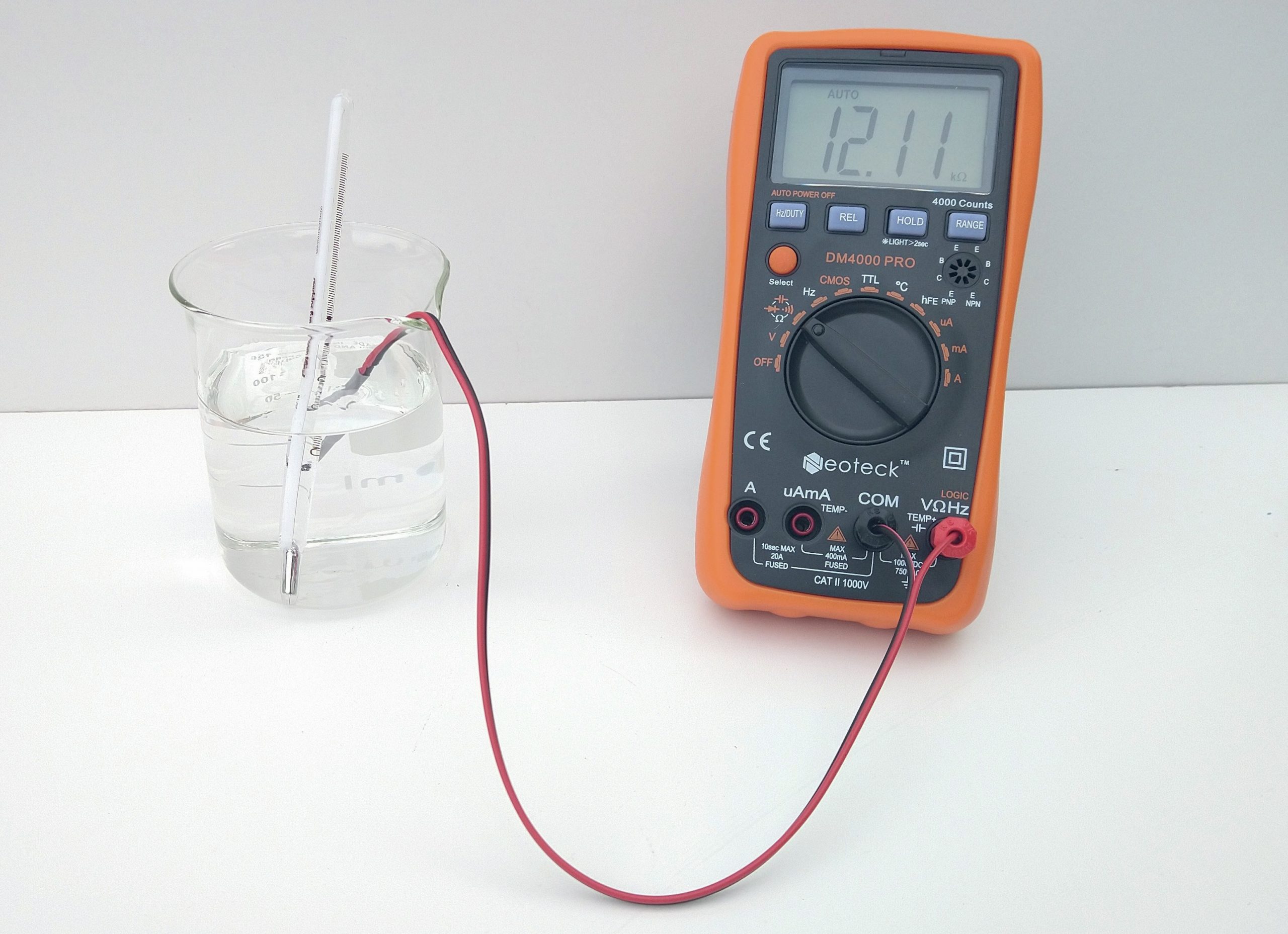
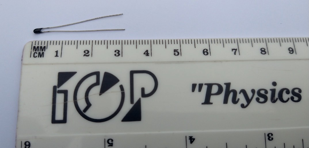
There are many possible thermistors available, but the one chosen for this experiment is a small bead-type NTC thermistor, with a nominal resistance of 15kΩ at 25°C. It will be immersed in a water bath, so the leads to the thermistor need to be well insulated in order to avoid errors caused by conduction through the water.
In order to obtain repeatable and precise measurements, the thermistor and a standard laboratory thermometer are put in a beaker of boiling water. The heater is removed and the resistance measured as the temperature of the water falls. The resistance is measured directly using a digital multimeter, although a voltmeter and ammeter can be used as an alternative. Make sure the current through the thermistor never exceeds a few milliamps, as too much current will cause heating of the thermistor, resulting in error.
Since using this method can require a long wait between measurements, this is an ideal use for a data-logger, to measure resistance and temperature over a period of a couple of hours. Temperatures below room temperature can be obtained by adding some ice to the water in the beaker.
Experimental results
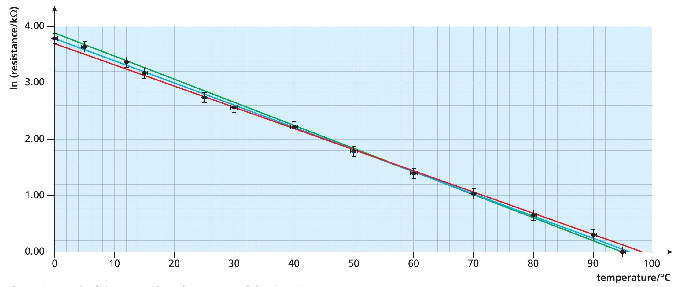
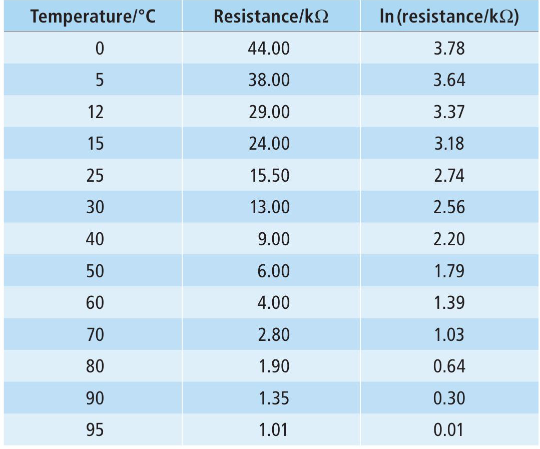
The resistance of the thermistor is measured at different temperatures between 100°C and 0°C. A typical set of results is shown in Table 1. Referring to Equation 2, we can plot a graph of lnR against T (Figure 1).
The gradient, m, of the best-fit line in Figure 1 gives:

The intercept, c, of this best-fit line on the y-axis is 3.8, so we have:
ln(R0/kΩ) = 3.8
R0/kΩ = e3.8
R0, best = 44.7kΩ
We can use these values of α and R0 in Equation 1 for calculating resistance RT at any temperature T.
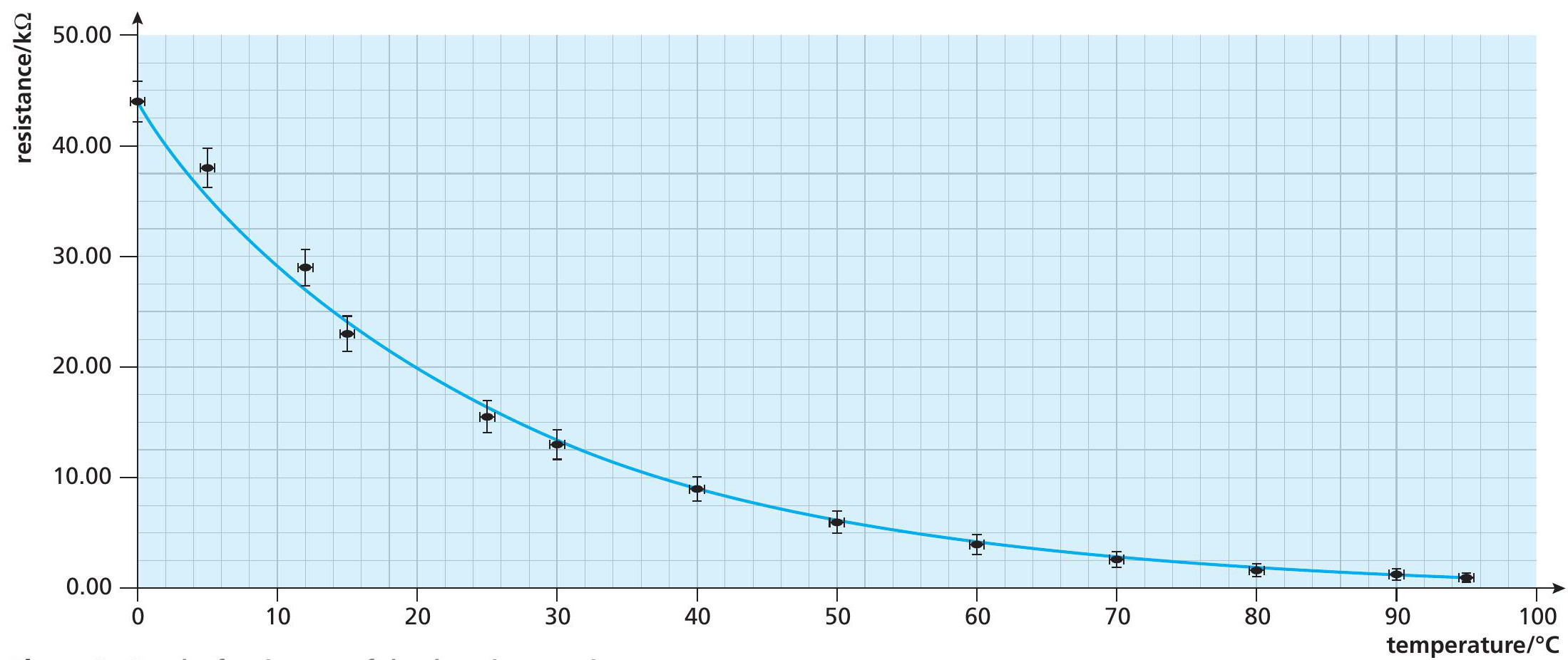
We can also use data from Table 1 to plot a graph of resistance against temperature (Figure 2). As expected from Equation 1, this does not give a straight line. By using a standard spreadsheet program, the equation of the best-fit line can be shown. In this case the program gives the equation of the best-fit line as:
RT = 44 × e−0.039T (5)
This gives values for R0 and α that are similar to the values found using the log graph in Figure 1. But note that Equation 5 is not the sort of equation that we usually write in physics, as it uses numbers without units, and only works if R is in kΩ and T in °C.
Uncertainty and error bars
The uncertainty in measuring the temperature, in this case with a laboratory thermometer, is ±0.5°C. Error bars corresponding to this uncertainty have been added to the graphs in Figures 1 and 2.
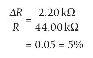
The uncertainty in the resistance measurement is more difficult to estimate because of the very wide range of resistance values. When several measurements were taken at 0°C, the range of values measured was between 41.8kΩ and 46.2kΩ, with an average value of 44.00kΩ. This range is 4.40kΩ, making the spread 2.20kΩ. This is a fractional uncertainty:
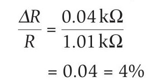
The range of resistances measured at 95°C was much smaller than at 0°C and was between 0.96kΩ and 1.04kΩ, giving a range of 0.08kΩ and so a spread of 0.04kΩ. With the average value of 1.01kΩ, this gives:
When plotting a natural log graph, the uncertainty in lnx is approximately equal to Δx/x provided that Δx << x. For all our resistance measurements, ΔR << R. Using the larger of the two percentage uncertainties, the error bars for lnRT are ±0.05, and these have been added to the graph in Figure 1.
Calculations
Using the error bars in Figure 1, the steepest possible line (green) and shallowest possible line (red) have been added. We can now complete the analysis using these lines to find the range of values for α and R0, and calculate the corresponding uncertainty in temperature.
The gradient of the steepest line (green) gives:
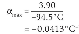
For this line the intercept on the y-axis,lnR 0 , is 3.9, which gives:
R0, max = 49.4kΩ
The gradient of the shallowest (red) line is:
The red line meets the y-axis where lnR is 3.7, which gives:
R0, min = 40.4kΩ
The gradients of the steepest and shallowest lines give a value for the uncertainty in ln T, but this is not the same as the uncertainty in T. These equations do not allow us to calculate an overall spread of values for temperature because they are simply the equations of the steepest and shallowest lines.
The spread of possible calculated values of temperature varies over the temperature range, with a minimum spread between 50°C and 60°C, where the lines cross. However, we can make a good estimate of the uncertainty in calculating temperature from a given resistance. When measuring the resistance at 0°C, the range of resistances measured was between 41.8kΩ and 46.2kΩ. Using these values in Equation 4 gives a range of calculated temperatures between –1.0°C and +2.0°C — a range of 3.0°C and a spread of ±1.5°C.
Summary
A reasonable conclusion from our calibration is that Equation 5, using the best-fit values of α (–0.0396 °C−1 ) and R0 (44.7kΩ) gives a value of temperature with an uncertainty of ±1.5°C.
Devices that use a thermistor to measure temperature will need to have a similar calibration equation built into their display in order to show an accurate temperature. Fortunately, modern electronic circuits make this a quite straightforward process.